The Google Sheet Assignment - Splitting and Transposing Cell based on Delimiter - Part 1

I recently had opportunity to workout a formula with google sheets, where i realized how powerful google sheet formulas are.

The problem consisted of following data:


.... To be converted this way:


The requirement was to identify the spaces in the in each cell in column B as a delimiter and separate the text based on that space, the corresponding value in the Column C was to be repeated the same number of time as was the space in the cell to left.

For example in Cell B2, the text contains two spaces, we will one more so that three words in the cell be repeated into three different cells.

As a first part, we will try to separate the text down the column:

The First Step is to Split the Values in Cells in Column B, for all cell in this column. For a single cell, the SPLIT will do the trick, for all the cells in the column, we will select the entire range of cells.

=TRANSPOSE(SPLIT(CONCATENATE(ARRAYFORMULA(SPLIT(INDIRECT("Sheet1!B$2:B"&COUNTA(Sheet1!B$1:B))," ")&" "))," "))

Using the Indirect function, we have made the selection dynamic, the resulting array is split cell wise into individual words.

With reference to our data, the COUNTA() function will return a value of 2 That will give result in range of B2:B2 provided to SPLIT() function that will return the following array:

{abc,defgh,ijkl20asdklj;asdlkejd,asdjkw,adkjw}

This array is provided to the CONCATENATE function that again converts it in to a single array:

{abc defgh jkl20asdklj asdlkejd asdjkw adkjw}

This is again split and then transposed to give the desired result.

So the basic resason for joining the two texts is to make sure that we don't have to find where the next part of the array from the second has to start, once we have concatenated everything, we can just split it based on a delimiter and then transpose to get the solution!

This split and concatenate function of google is enough to made any one mad who has worked with MS Excel's concatenate function that required fixed cells to be feed to it, however this short coming is overcomes in later versions of excel, but still, google sheet is far more ahead in terms of functionality that G sheet provides.

The ArrayFormula makes sure that we don't need to copy paste it over and over again! again a feature missing in MS Excel.

Can you create acronyms from a list in Excel Sheet?

Can you crate the acronyms in Excel? If you are given a set of Strings and be asked to create the acronyms how will you proceed. My today's post is related to creating acronyms!!

Lets consider a list of string like one given here  (and adopted from here):


The formula we need to built will work by identifying the the characters followed by spaces, we will add a space to the start of each string. If the strings are present in Column A, the new string will be:

=" "&String

... and the table will look like:


You can see the extra space at the start of the string in Column D, now we can use this extra space as a delimiter and convert text-to-column operation, the operation results in words being placed in the individual columns:


Now we can get the first character of each individual word in the cell by using the formula =PROPER(LEFT(Cell_Ref)). We can simply put it in a cell below the table and drag to right and down to get another table. Here it is...


We can use now, the built in concatenate or any udf available from the internet. If we just keep it an ampersand sign, we can do it like this to get the desired result.

=TRIM(E18&F18&G18&H18&I18&J18&K18)

Obvisouly if it is a repetitive task, you can create a udf of your own or a macro to finish the task. This was just a quick tutorial to show how to do it. If you like it do share and comment. 

Survival Analysis with Kaplan-Meier Method

My today’s post is about Survival Analysis with Kaplan-Meier Method.

This post uses an example for a popular multivariate analysis textbook to emulate the problem and hence providing and excel based solution to it. For this post our point of focus will be how to emulate the analysis on Excel rather than theory. For theory there is several standard text available that can used for understanding theory behind the method.

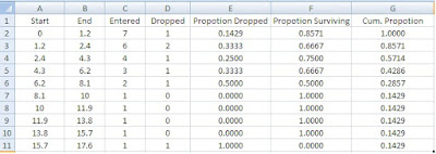
The method we are discussing is Kaplan-Meier Method. The key is to make a table with survival data and then process with the calculations involved.


Interval Start: 

The first Cell is entered manually; rest equals the end interval of the upper group. Say for group 2, the start interval is equal to end interval of group 1. (A3 = B2)

Interval End: 

Start interval of the corresponding group multiplied by 2 to give end interval. For first group it is manually entered. 

Entered and Dropped: 

These are from your observational data. This basically described how many patients entered the time bracket we are considering for example for the first group, time bracket is from 0 to 1.2 month. For this group 7 in Entered means those 7 patients were admitted at the start of this group. Whereas 1 in dropped means that by the end of 1.2 months, 01 patient was lost or withdrew from the observation, thus only 6 patients entered the next time bracket o f 1.2 - 2.4 months. 

Proportion Dropped: 

This is calculated by no. of dropout divided by total number entered for a an interval. For our case it is D2/C2

Proportion Surviving: 

This is simply 1-(D2/C2) or for out sheet 1-E2, theoretically it is ..

$$Proportion Surviving=\frac{Total Patients - Dropouts}{Total Patients}$$

Cumulative Proportion: 

This stands for cumulative proportion surviving and this is of actual interest to most of the people. Formula for this is:

$$Cumulative Proportion=\frac{Patients Survived for till an Interval}{Total Dropouts}$$

For our case the formula is =C2/SUM($D$2:$D$11)

Creating a Graph:

For K-M Estimator, the standard graph is a stair-case like graph, but for the sake of simplicity and ease of use, a simple scatter plot can do the trick. 


With this chart you can add a trend. For trend lines, if our data starts with zero, we cannot use power and logarithmic trends lines, hence I have used polynomial line with 3 – degree and it is displayed as equation in the graph.

In the next post I will explain how to calculate the hazard function and density function and standard error for the survival analysis. You can download workbook from this link.

Analyzing Performance of Your Purchase Department with Excel®

A recent situation created in my office when a vendor rushed into my office and started shouting. He was annoyed by the non-serious behavior of our purchasing staff. When my boss started addressing his grievances he claimed that his payments have been pending for long period of time, even more then the credit period in the purchase order.

The situation was later analyzed to see who actually is responsible for the delay in payments. So we started by answering following question:

How much amount in Rs. is pending?
How many bills are pending for payment?
How much amount (and bills) is actually due by now?
What is the share of each purchaser

We start with the following dummy data, just few entries to elaborate the process. (The data has been produced using DK Data Generator, freely available from internet).


Creating the Basic Table  

Q1    =SUMPRODUCT(($E$6:$E$20=B23)*($C$6:$C$20))
Q2    =SUMPRODUCT(($E$6:$E$20=B23)*1)
Q3    =SUMPRODUCT(($E$6:$E$20=B23)*($F$6:$F$20="DUE")*($C$6:$C$20))
Q4    =SUMPRODUCT(($E$6:$E$20=B23)*($F$6:$F$20="DUE")*1)


Creating Frequency Bin:
 

A frequency charts simply a frequency histogram to plot the situation. Following formulas has been used.

Getting Count    =SUMPRODUCT(($G$6:$G$20>=C30)*($G$6:$G$20<=D30)*1)
Creating Bars    =REPT("g",E30)


Interpretation:

The interpretation is easy. You can see that out of the total outstanding bills to be paid, Mr. A has contributed the most in accumulating these bills. While Mr. D is leading for the case of the bills that are actually due and need to be paid. Both of these guys need to work really hard over billing. The histogram reveals another critical piece of information. Most of the bills have been dealed well over the credit limit i.e. 45 days. The avg. pending time is about 150 days (because this is not an ideal bell-shaped curve and the histogram is more looks a square). So we can understand why people rushed in our office and shouted.

Download the File: Store Performance 

Hope that this posts explained something useful! Take care

Using Text() function to test your Custom Number Formatting


The feature that custom number formatting (from now onward CNF) offers has been discussed on various website in very detail. One of the webpage that I like most is by Tom Niche that has a very detailed post on this feature of excel. In this post I will explain how you should proceed with various features of CNF to get a desired result. 

For the sake of elaboration I will take up few examples:

Example 01:    INDIAN/PAKISTANI CURRENCY FORMAT

The Asian subcontinent traditionally measure monetary wealth in Thousand, Lacs, Carrors instead of Million, Billion and Trillion Rupees. The difference become apparent when you write a number in two different formats like below: 

Amount
Indian
Non-Indian
100000/-
100,000/-
100,000/-
1000000/-                        
10,00,000/-
1000,000/-
10000000/-                      
100,00,000/-
10,000,000/-
100000000/-                   
10,00,00,000/-
100,000,000/-

The difference between two can be observed while observing the placement of comma (,) in the numbers. Up till amount of 0.1 Million, both follows same patron but above this value, the Non-Indian System groups digits in bunch of three, while the Indian system groups the first three digits (the thousandth part) into three digits and remaining into the groups of two digit each. So the question is how we are going to create a CNF that corresponds to our Indian Requirement. 

Fortunately most of the format has already been created by experts. We just need to understand how they work, rather what is the principle that is used in their making. Let’s start with our requirement. We want to have a 7 digits number that follows the Indian format. For our case can write this number this way:

#
#
\,
#
#
\,
#
#
#

Now your custom format is ready for use. Try it on an excel sheet. But your CNF is still not ready to use. If with this format you try to write a five digit number, the format will place one comma before the number. For example if you write 12500, it will appear as [,12,500] so what we need to do is to place some sought of condition that can be checked for and then CNF applied. That condition is added like this:

If a number is less then 05 digits
####0.00
If a number is greater then 05 digits
[>99999]##\,###0.00
If a number is greater then 07 digits
[>9999999]##\,##\,###0.00

Putting all this stuff together we can find reach this complete criterion. 

[>9999999]#\,##\,###0.00; [>99999]#\,###0.00; ###0.00

Thus we have reached our desired format. 

But there is a limitation to this process!! As I tried to add another level of detail to the above CNF, Excel informed me that I need to try a built in format for that! So what should then we can do it then? My suggestion is to make us of Text() function in excel. The idea is to create a lookup table with desired output format and criteria’s.

Situation
Criteria
Format
If a num > 03 digits
999
#\,##0.00
If a num > 05 digits
99999
#\,##\,##0.00
If a num > 07 digits
9999999
#\,##\,##\,##0.00
If a num > 09 digits
999999999
#\,##\,##\,##\,##0.00

Practically it might not be possible to have a lookup table and do this stuff. This was just meant for theoretical understanding. However this idea of having a table can be handy when you want to check custom number formats of your own.

Running Simple Linear Regression on Eviews

In this post I will be explaining how to run the Simple Linear Regression (Ordinary Least Square) to create the model using Eviews 7.0. Eviews is especially strong in analysis of time series data so for the purpose of elaborating the process we will be using the time series data of the GTI and Remittance of Pakistan for last thirty years from 1981 to 2010.

The process starts by opening a new file of Eviews. Here are the steps:

1. Open the new Eviews File.


2. Specify the time period from 1981 to 2010.

3. Now specify the variables, rem for remittance and gti for grand total investment. Write data rem gti in the space provided for this purpose.
 

4. This will make a table that will have space for the two variables, now copy and paste the data from excel sheet to this table.


5. Now go to Quick, Equation Estimate and write the expression defining the relation between the two variables. Write: gti c rem


6.  Press ok to run the test. The results are viewed in a separate window. So here are the results:

RESULTS

Dependent Variable: GTI


Method: Least Squares


Date: 01/08/14   Time: 11:39


Sample: 1981 2010


Included observations: 30


Variable
Coefficient
Std. Error
t-Statistic
Prob.  


C
1008870.
335774.6
3.004605
0.0056
REM
-66900.59
59901.53
-1.116843
0.2736


R-squared
0.042648
    Mean dependent var
665670.2
Adjusted R-squared
0.008457
    S.D. dependent var
744393.0
S.E. of regression
741238.7
    Akaike info criterion
29.93437
Sum squared resid
1.54E+13
    Schwarz criterion
30.02779
Log likelihood
-447.0156
    Hannan-Quinn criter.
29.96426
F-statistic
1.247338
    Durbin-Watson stat
0.095653
Prob(F-statistic)
0.273554


Interpretation of Results:

The equation can be formed using the coefficients. In our case it will be GTI = 1008870 – 66900.59 REM.     

Prob. Value explains that percentage of error in the coefficients, C has 0.56% error while REM has 27.36% error. R-Squared value states that our model is explained 4% by this equation (this is really undesirable; we need this value to be 50%+ range). F-Statics explains the combined effect of two variables and Prob (F-Statistic) states there are 27% chances of error in this estimate. Durbin Watson stat explains the autocorrelation exists on at 0.09; we can use LM Test to further confirm its existence.

Overall the model is poorly explained by the regression line, in such a case we either need to add more independent variables that explain further the relationship or take data for a longer time period to examine the relation. This was all about the post. You can download the sample files and try at your end.


Download EViews Sample File from here.

The Google Sheet Assignment - Splitting and Transposing Cell based on Delimiter - Part 1

I recently had opportunity to workout a formula with google sheets, where i realized how powerful google sheet formulas are. The problem ...